Science study
Plot a science graph: axes, scale and best fit
Turn a results table into a readable graph, then check what the points actually support. Work through an original example on paper.

You have a results table, a ruler and an empty grid. When you plot a science graph, the difficult part is often deciding what the picture should mean. Which variable belongs on each axis? How much does a small square represent? Should the points be joined, or should you draw a line that describes their overall pattern? Making those decisions before drawing saves more time than starting with the nearest available scale.
This guide uses invented measurements for practice, not observations from a real experiment. You can complete the whole task for free with paper and a pencil; no account or paid plotting service is needed. Keep your actual assignment beside the grid because its instructions may specify the axes, plotting symbols or type of line. A graph communicates evidence. It cannot supply a missing measurement, prove a cause by itself or guarantee a particular mark.
1. Plot a science graph for the question you were asked
First identify the requested output. A task asking you to display changes over time differs from one asking you to investigate a relationship between two measured quantities. Read whether it asks for a bar chart, a scatter graph, a straight line of best fit or a smooth curve. Do not choose a familiar shape simply because it is easy to draw. Categories such as three different materials usually need a different display from a continuous variable such as time.
For our practice example, imagine a results table listing time in seconds and distance in centimetres. The pairs are (0, 2), (10, 7), (20, 11), (30, 17), (40, 22) and (50, 26). These values were chosen to practise plotting a roughly straight trend with some scatter. They are not a claim about a particular object or experiment. The task is to show distance against time and estimate the overall relationship, rather than describe each reading as an exact law.
Write a small plan above your working notes: horizontal quantity, vertical quantity, minimum and maximum values, and required line. If the question gives a fixed grid, count its usable squares before drawing. Our separate guide to a lab-report conclusion is useful when the final task asks what your graph supports. Keeping the graph question separate from the conclusion prevents you from drawing the result you hoped to see.
2. Give every axis a quantity and a unit
In a typical school experiment, the quantity you change or choose goes on the horizontal x-axis and the response you measure goes on the vertical y-axis. For the invented table, write time (s) along x and distance (cm) along y. Time is the chosen observation coordinate; distance is the reported response. Some assignments reverse the usual order or supply specific axis labels, so follow the actual question rather than a memorised rule about whichever column appears first.
A label such as x or results tells a reader too little. The quantity and unit should make each coordinate meaningful without access to your notebook. A point at (20, 11) then means a distance of 11 cm at 20 s. If one row uses metres and the rest use centimetres, convert consistently in a working table before plotting. Keep the original values available so you can check the conversion rather than silently replacing the evidence.
Qualifications Scotland’s scientific graphing guidance explains how axes, quantities and units make experimental data readable. Use that free reference to check those conventions, while keeping our original data for practice. Write a descriptive title such as Distance against time for the practice data. A title identifies the relationship; it should not announce that a hypothesis has been proved before you have interpreted the points.
3. Choose scales you can read and reproduce
Look at the largest values before numbering the axes: 50 s horizontally and 26 cm vertically. Suppose your working area allows 25 small squares in each direction. A horizontal scale of 2 s per small square covers 50 s. A vertical scale of 2 cm per small square covers 50 cm, leaving more space than needed; 1 cm per square would not fit 26 cm. You could instead use a taller grid with 30 squares and 1 cm per square. The physical grid matters.
Choose simple increments that make the coordinate of each small square clear. Steps of 1, 2 or 5 units, multiplied by a suitable power of ten, are usually easier to read than awkward fractions. Label major ticks regularly and keep equal numerical differences equally spaced on each linear axis. The two axes do not need the same numerical scale. Two seconds horizontally and one centimetre vertically are different quantities, not a contradiction.
Do not squeeze all points into one corner or let the final value fall outside the grid. Leave room for labels and a sensible margin. An axis need not always begin at zero, but any shortened range must be clear and permitted by the task. Never write evenly spaced numbers such as 0, 10, 20, 50 on a linear axis. That makes the drawing inconsistent even if the points look tidy. Recheck the labels before adding the first mark.
4. Plot one pair at a time, then reverse the check
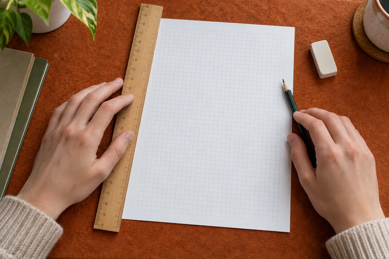
Locate each point by moving across to its x-value and up to its y-value. With 2 s per horizontal square and 1 cm per vertical square on a suitable grid, (20, 11) lies ten squares across and eleven squares up. The point (10, 7) lies five across and seven up. Use the small, clear plotting symbol requested by your teacher. A thick blob can hide an error of several squares and make later readings less precise.
Work through the table in order and mark each row as plotted in your notes. Unequal times must have unequal horizontal gaps. If the table instead listed 0, 10, 25 and 50 s, the points should not be evenly distributed just because there are four rows. The axis measures time, not the row number. Missing readings stay missing; you cannot add a point at an unmeasured time merely to fill a visual gap.
After plotting, read the coordinates back from the graph without looking at the table, then compare them. This reverse check catches swapped axes and scale errors. For our final point, you should recover approximately 50 s and 26 cm. Also count the plotted observations against the six pairs. Keep any uncertainty information supplied by the task, but do not invent error bars or a measurement resolution that the original table does not state.
5. Decide what the line represents
A line joining consecutive observations shows the sequence between those readings; it is not automatically a fitted model. A line of best fit describes an overall relationship in a scatter of experimental points. Read the instruction again before choosing. If a straight fit is requested and the pattern supports it, aim for a sensible balance of points around the line across the full range. Do not zigzag through every point and call that a straight fit.
Our values are broadly consistent with a line near distance = 2 + 0.5 × time, using centimetres and seconds. At 20 s that line gives 12 cm, while the invented observation is 11 cm; at 30 s it gives 17 cm. These differences illustrate scatter, not permission to alter the table. The relationship has an intercept near 2 cm. Forcing the line through (0, 0) would ignore the initial value, so zero should not be added as a fictional observation.
A visibly curved pattern calls for the type of curve required by the assignment, not a straight line chosen for convenience. If no relationship is clear, describe that limit instead of manufacturing one. The shared Lirno card is optional support; this paper method stands on its own. If you later use a targeted explanation in the tutor, ask about your specific choice of line rather than requesting a replacement graph to copy.

6. Investigate an unusual point without deleting evidence
Suppose a second practice table gives 39 cm at 30 s instead of 17 cm. Plot it accurately first. It lies well away from the trend, but appearance alone does not tell you why. Check the original row, unit conversion, plotted coordinates and measuring procedure. A copied digit or mistaken scale is a correctable recording or plotting error; a genuine unusual observation requires a different discussion. Keep a record of any correction and its reason.
Do not erase a point simply because it makes the fit less attractive. If the task allows a suspected anomaly to be excluded from a fit, leave the observation visible and explain the evidence for treating it separately. You might note that a repeat measurement is needed. With only six observations, one unusual point can matter substantially, so report the uncertainty instead of promising that the remaining line is the true behaviour of the system.
7. Read estimates and gradients with their limits
Reading inside the measured range is interpolation. On the illustrative line above, 25 s corresponds to about 14.5 cm. This is an estimate from the model, not an additional measurement. Extending the same line to 80 s would predict about 42 cm, but that is extrapolation beyond our table. The relationship may change there. State the difference whenever you report a value; a neat line does not remove the uncertainty outside the observed range.
If a gradient is requested for a straight best-fit line, select two well-separated positions on that line. They need not be original plotted observations. For line positions (10 s, 7 cm) and (40 s, 22 cm), the gradient is (22 − 7) / (40 − 10) = 0.5 cm/s. Write the changes in quantities and the units, not just a triangle drawn on the paper. Reversing the numerator and denominator changes both the number and the meaning.
Keep the conclusion proportional to the evidence. In this invented example the graph suggests that distance increases roughly steadily with time over the displayed interval. It does not establish why, or show that the same relationship continues indefinitely. For a curved line, the gradient varies with position, so a single large triangle is not automatically an instantaneous rate. Follow the required method and do not turn a general plotting exercise into an unsupported physical claim.
8. Make a second graph to test your decisions
For free science graph practice, reuse the original six pairs but choose a different valid grid. Can you explain each small-square value, plot the pairs and read them back? Then try the uneven times 0, 10, 25 and 50 with distances 2, 7, 15 and 26. This new invented set tests spacing. A friend should be able to recover the quantities and units without your explanation. If they cannot, revise the labels rather than adding decorative detail.
Turn any recurring error into a focused exercise. If scales are difficult, practise only selecting ranges on three empty grids before plotting. If axes are reversed, write the relationship in words first. The study-practice workflow describes an optional way to revisit ideas, but a paper attempt and reverse check already give you a complete starting method. Lirno is free to download or start; some AI usage levels or advanced features may require Premium.
If you use AI to discuss a graph, verify the captured table, units, axis labels and full instructions yourself. AI can misread a decimal or reason incorrectly. Your school’s rules still apply, and Lirno does not guarantee correctness, grades, mastery or permission to use assistance. Submit a graph you can explain: why those axes, why that scale, which values were measured, what the line means and where its interpretation stops.